Excel logical formulas: 8 simple IF statements to get started

Excel functions, or formulas, lie at the heart of the application’s deep well of capabilities. Today we’ll tackle IF statements, a string of commands that determine whether a condition is met or not. Just like a yes-no question, if the specified condition is true, Excel returns one user-determined value and, if false, it returns another.

The IF statement is also known as a logical formula: IF, then, else. If something is true, then do this, else/otherwise do that. For example, if it’s raining, then close the windows, else/otherwise leave the windows open.

The syntax (or sentence structure; that is, the way the commands are organized in the formula) of an Excel IF statement is: =IF(logic_test, value_if true, value_if_false). IF statements are used in all programming languages and, although the syntax may vary slightly, the function provides the same results.

Past-due notices

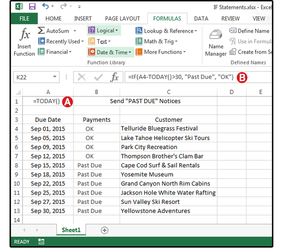
In this spreadsheet, the customer’s payment due date is listed in column A, the payment status is shown in column B, and the customer’s company name is in column C. The company accountant enters the date that each payment arrives, which generates this Excel spreadsheet. The bookkeeper enters a formula in column B that calculates which customers are more than 30 days past due, then sends late notices accordingly.

A. Enter the formula: =TODAY() in cell A1, which displays as the current date.

B. Enter the formula: =IF(A4-TODAY()>30, “Past Due”, “OK”) in cell B4.

In English, this formula means: If the date in cell A4 minus today’s date is greater than 30 days, then enter the words ‘Past Due’ in cell B4, else/otherwise enter the word ‘OK.’ Copy this formula from B4 to B5 through B13.

Pass/Fail lifeguard test

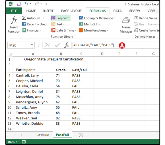
The Oregon Lifeguard Certification is a Pass/Fail test that requires participants to meet a minimum number of qualifications to pass. Scores of less than 70 percent fail, and those scores greater than that, pass. Column A lists the participants’ names; column B shows their scores; and column C displays whether they passed or failed the course. The information in column C is attained by using an IF statement.

Once the formulas are entered, you can continue to reuse this spreadsheet forever. Just change the names at the beginning of each quarter, enter the new grades at the end of each quarter, and Excel calculates the results.

A. Enter this formula in cell C4: =IF(B4<70,”FAIL”,”PASS”). This means if the score in B4 is less than 70, then enter the word FAIL in cell B4, else/otherwise enter the word PASS. Copy this formula from C4 to C5 through C13.

Sales & bonus commissions

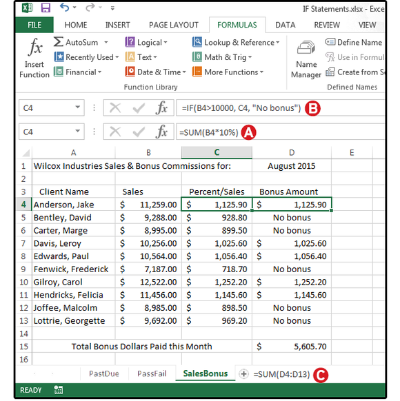
Wilcox Industries pays its sales staff a 10-percent commission for all sales greater than $10,000. Sales below this amount do not receive a bonus. The names of the sales staff are listed in column A. Enter each person’s total monthly sales in column B. Column C multiples the total sales by 10 percent, and column D displays the commission amount or the words ‘No Bonus.’ Now you can add the eligible commissions in column D and find out how much money was paid out in bonuses for the month of August.

A. Enter this formula in cell C4: =SUM(B4*10%), then copy from C4 to C5 through C13. This formula calculates 10 percent of each person’s sales.

B. Enter this formula in cell D4: =IF(B4>10000, C4, “No bonus”), then copy from D4 to D5 through D13. This formula copies the percentage from column C for sales greater than $10,000 or the words ‘No Bonus’ for sales less than $10,000 into column D.

C. Enter this formula in cell D15: =SUM(D4:D13). This formula sums the total bonus dollars for the current month.

Convert scores to grades with nested IF statements

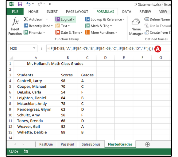
This example uses a “nested” IF statement to convert the numerical Math scores to letter grades. The syntax for a nested IF statement is this: IF data is true, then do this; IF data is true, then do this; IF data is true, then do this; IF data is true, then do this; else/otherwise do that. You can nest up to seven IF functions.

The student’s names are listed in column A; numerical scores in Column B; and the letter grades in column C, which are calculated by a nested IF statement.

A. Enter this formula in cell C4: =IF(B4>89,”A”,IF(B4>79,”B”,IF(B4>69,”C”,IF(B4>59,”D”,”F”)))), then copy from C4 to C5 through C13.

Note: Every open, left parenthesis in a formula must have a matching closed, right parenthesis. If your formula returns an error, count your parentheses.

Determine sliding scale sales commissions with nested IF statements

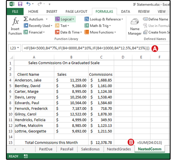
This last example uses another nested IF statement to calculate multiple commission percentages based on a sliding scale, then totals the commissions for the month. The syntax for a nested IF statement is this: IF data is true, then do this; IF data is true, then do this; IF data is true, then do this; else/otherwise do that. The names of the sales staff are listed in column A; each person’s total monthly sales are in column B; and the commissions are in column C, which are calculated by a nested IF statement, then totaled at the bottom of that column (in cell C15).

A. Enter this formula in cell C4: =IF(B4<5000,B4*7%,IF(B4<8000,B4*10%,IF(B4<10000,B4*12.5%,B4*15%))), then copy from C4 to C5 through C13.

B. Enter this formula in cell C15: =SUM(C4:C13). This formula sums the total commission dollars for the current month.

Calculate product price based on quantity

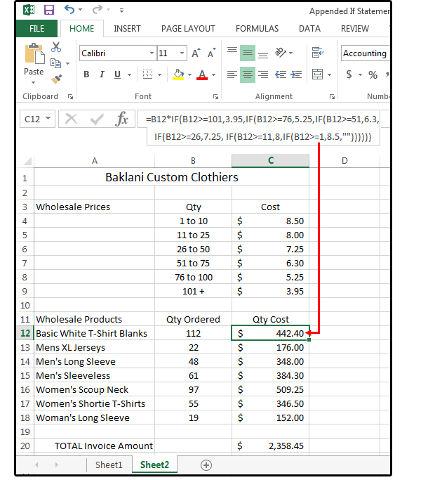
Many retailers and most wholesalers provide customers a price break based on quantity. For example, a wholesaler may sell 1 to 10 T-shirts for $10.50 each, and 11 to 25 T-shirts for $8.75 each. Use the following IF statement formula to determine how much money you can save by purchasing wholesale products for your company in bulk.

1. Enter the header Wholesale Prices in cell A3. Enter the headers Qty and Cost in cells B3 and C3.

2. Enter the quantity breaks in cells B4 through B9.

3. Enter the price breaks in cells C4 through C9.

This is the quantity/price matrix for your wholesale business.

4. Next, enter the headers Qty Ordered and Qty Cost in cells B11 and C11.

5. Enter the header Wholesale Products in cell A11, then enter as many products as you like below.

6. Enter the quantity ordered for each product in column B.

7. And last, enter the following formula in the adjacent cells of column C:

=B12*IF(B12>=101,3.95,IF(B12>=76,5.25,IF(B12>=51,6.3,IF(B12>=26,7.25, IF(B12>=11,8,IF(B12>=1,8.5,””))))))

Note there are no spaces in this formula. Copy down the formula as far as needed in column C to apply to all the wholesale products and quantities in columns A and B.

8. Once the order is complete, create a total line: In column A (in this case, A20), type TOTAL Invoice Amount. In column C (in this case, C20), use the SUM function to total the column.

Now, that all the formulas are in place, all you have to do each week (or month) is enter the new quantities in column B, and Excel does the rest. If the prices change, just modify the matrix at the top of the spreadsheet, and all the other formulas and totals will automatically adjust.

Using other functions inside the IF statement

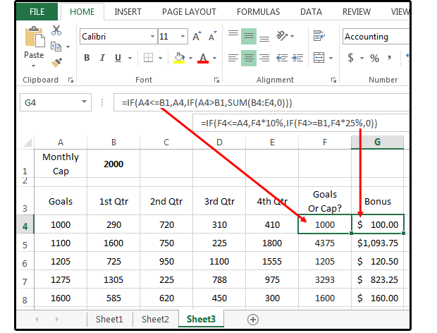
In this example, we’ll nest two IF statements and insert the SUM function all into the same formula. The purpose is to determine whether the individual’s goals are less than, equal to, or greater than the company’s monthly cap.

1. Enter a monthly cap amount in B1, which can be changed every month to reflect the company’s expectations.

2. Enter the following headers in cells A3 through G3: Goals, 1st Qtr, 2nd Qtr, 3d Qtr, 4th Qtr, Goals or Cap?, and Bonus.

3. Enter the top five marketing persons’ goal amounts in cells A4 through A8.

4. Enter the same individuals’ quarterly totals in cells B4 through E8.

PC World / JD Sartain

For employees who achieved their goals, the bonus is 10% of the goal amount. For employees who exceeded the monthly cap, the bonus is 25% of their actual sales. Use these formulas to determine the bonus amounts.

5. Enter this formula in cells F4 through F8: =IF(A4<=B1,A4,IF(A4>B1,SUM(B4:E4,0)))

6. Enter this formula in cells G4 through G8: =IF(F4<=A4,F4*10%,IF(F4>=B1,F4*25%,0))

Use IF to avoid dividing by zero

In Excel, if you try to divide any number by zero, the error message that Excel displays is this: #DIV/0!

So, what to do if you have a large database that requires a calculation based on division, and some of the cells contain zeros? Use the following IF statement formula to address this problem.

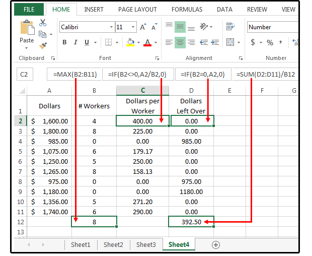
1. To track the money collected per month by the staff at Friar Tuck’s Fundraisers, open a spreadsheet and create the following headers: Dollars in A1, Dollars per Worker in B1, Dollars Left Over in C1.

2. Enter some dollar amounts in column A and the number of staff working per day in column B. Column B will include some zeroes because, some days, nobody works (but donations still come in through the mail).

2. Enter this formula in C2 through C11: =IF(B2<>0,A2/B2,0). By using an IF statement to prevent Excel from dividing any of the funds collected by zero, only the valid numbers are calculated.

PC World / JD Sartain

3. You could use another IF statement to locate the zeroes in column B, then total the corresponding dollars in column A, which would then be divided equally among all the staff. Copy this formula in D2 through D11: =IF(B4=0,A4,0).

4. Next, move your cursor to B12 and enter this formula =MAX(B2:B11) to locate the largest number of workers in column B, which is eight.

5. Move your cursor to D12 and enter this formula: =SUM(D2:D11)/B12. The answer is $392.50 for each of the eight staff members working at Friar Tuck’s Fundraisers.

Editor’s note: This article was updated from its original posting on September 8, 2015.