The bigger and uglier your Excel spreadsheet gets, the more you need to use certain features or tricks to keep a handle on the data. The seven features covered here will help you navigate, organize, and readjust your spreadsheet with as little hassle as possible.

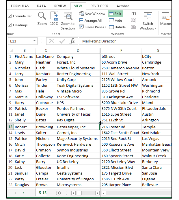
1. Split Screen

One of the most helpful features for large spreadsheets is the Split Screen command. The Split Screen allows you to view two, three, or four windows of your spreadsheet. Use this feature to work on one section of your spreadsheet while you view another section; or use it to compare (side by side) two sections of the spreadsheet. Once you try it, you’ll find lots of reasons to use it.

a. First, position your cursor where you’d like the screen to split. For example, if you want to divide the screen into four equal sections, position the cursor in the center of the spreadsheet.

b. Next, select View > Split. Notice the screen splits into four equal sections.

c. If you want to move the split, position your cursor at the apex of the split bars. When the cross with arrow points appears, click and hold, then drag the cross with arrow points across the screen until the screen is divided to your satisfaction.

d. To remove the Split, click View > Split (again).

JD Sartain

2. Freeze Frames

The other great feature for large spreadsheets is Freeze Frames. People generally freeze frames so they can see the column headers as they scroll down the page, or the first row as they scroll across, as they usually contain the spreadsheet’s unique fields such as client name, part number, or item number. Use the following instructions to freeze columns A and B (first and last name) and row 1, the field names (column headers).

a. Position your cursor on cell C2.

b. Click View > Freeze Frames > Freeze Frames. Notice that Excel inserts a thin line below row 1 and to the right of column B.

c. Cursor down, and all the rows scroll up except row 1. Cursor right, and columns A and B are stationary, while the remaining columns move to the left.

d. Now when you update the fees in column K, you can see the names of the individuals who owe those fees.

[Source”timesofindia”]